The simplest functions are lineal functions. Their formulas are polynomials with degree one or cero (this is the
case when the function is the constant function). Their graphs are straight lines.
A formula for these lineal functions is:
We usually call it the slope-intercept form, where b is the y-intercept and m is the slope.
The slope, also called the gradient of the line, measures the degree of inclination of the line with the horizontal, the x-axis.
The slope of a line characterizes the general direction in which a line points.
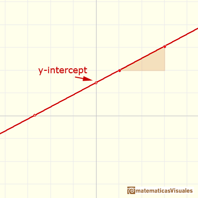
The y-intercept of a function is the point at which the graph of the function
crosses the y-axis. (the x value equals 0 ). The y-intercept of a linear function is:
When b is positive, the line crosses the y-axis somewhere above the x-axis (y=0) and if b is negative,
the line crosses the y-axis below the x-axis.
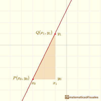
A line is completely determined by any two distinct points along it. If (x0, y0) and
(x1, y1) are two points (x0 not equal x1) on a given line we can calculate the slope of the line:
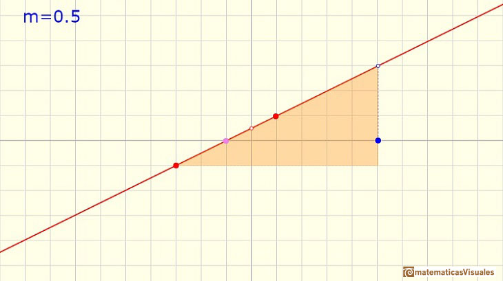
Notice that when the slope, m, is positive, the line slants upward to the right. The more positive m is,
the steeper the line will
slant upward to the right.
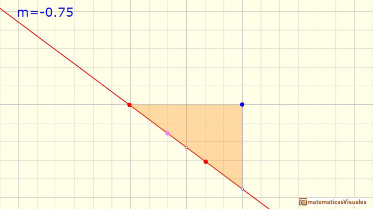
When the slope is negative, the line slants downward to the right, and, as the slope becomes
more and more negative, the line will slant downward steeper and steeper to the right.
This is an example of a linear function with a negative slope:
Horizontal lines have slope=0. All horizontal lines are of the form y = k (where k is some number).
As a function, we call it a constant function.
Vertical lines have no slope. They are not function at all. Note that if we try to calculate the slope we end up trying to
divide by 0.
In applications, if we know that the functional
relation between the variables is characterized by a
constant rate of change, then the underlying
function is linear and its slope measures this rate of
change. This information can be exploited to write
down a formula for the function.
The line thorugh P(x0, y0) with slope m is given by the point-slope form:
We can rearrange to write it as a function:
We can write the equation of the line though two points:
That has the advantage that we do not need to divide. We can arrive at the general form
(this algebraic form has an important advantage because it include vertical lines x = k, where k is some real number):
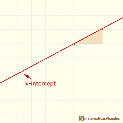
The x-intercept of a linear function is the point where the graph of the line crosses the x-axis. A non-horizontal line always have one x-intercept.
To find the x-intercept we need to solve the equation
This solution of the equation is called a root of the polynomial. In general, a function can have several x-intercepts.
Then the x-intercept of a linear function (with m not equal to 0) is:
The simplest example of a Lagrange Polynomial is, of course, the linear function through two points. We can write this linear function
as a simple example of a Lagrange Polynomial:
MORE LINKS

Power with natural exponents are simple and important functions. Their inverse functions are power with rational exponents (a radical or a nth root)

Polynomials of degree 3 are cubic functions. A real cubic function always crosses the x-axis at least once.

We can consider the polynomial function that passes through a series of points of the plane. This is an interpolation problem that is solved here using the Lagrange interpolating polynomial.

The derivative of a lineal function is a constant function.

The derivative of a quadratic function is a linear function, it is to say, a straight line.

The derivative of a cubic function is a quadratic function, a parabola.

Lagrange polynomials are polynomials that pases through n given points. We use Lagrange polynomials to explore a general polynomial function and its derivative.

If the derivative of F(x) is f(x), then we say that an indefinite integral of f(x) with respect to x is F(x). We also say that F is an antiderivative or a primitive function of f.

The integral concept is associate to the concept of area. We began considering the area limited by the graph of a function and the x-axis between two vertical lines.

Monotonic functions in a closed interval are integrable. In these cases we can bound the error we make when approximating the integral using rectangles.

If we consider the lower limit of integration a as fixed and if we can calculate the integral for different values of the upper limit of integration b then we can define a new function: an indefinite integral of f.

It is easy to calculate the area under a straight line. This is the first example of integration that allows us to understand the idea and to introduce several basic concepts: integral as area, limits of integration, positive and negative areas.

To calculate the area under a parabola is more difficult than to calculate the area under a linear function. We show how to approximate this area using rectangles and that the integral function of a polynomial of degree 2 is a polynomial of degree 3.

We can see some basic concepts about integration applied to a general polynomial function. Integral functions of polynomial functions are polynomial functions with one degree more than the original function.

The Fundamental Theorem of Calculus tell us that every continuous function has an antiderivative and shows how to construct one using the integral.

The Second Fundamental Theorem of Calculus is a powerful tool for evaluating definite integral (if we know an antiderivative of the function).

As an introduction to Piecewise Linear Functions we study linear functions restricted to an open interval: their graphs are like segments.

A piecewise function is a function that is defined by several subfunctions. If each piece is a constant function then the piecewise function is called Piecewise constant function or Step function.

A continuous piecewise linear function is defined by several segments or rays connected, without jumps between them.

By increasing the degree, Taylor polynomial approximates the exponential function more and more.

By increasing the degree, Taylor polynomial approximates the sine function more and more.

Complex power functions with natural exponent have a zero (or root) of multiplicity n in the origin.

A polynomial of degree 2 has two zeros or roots. In this representation you can see Cassini ovals and a lemniscate.

A complex polinomial of degree 3 has three roots or zeros.

Every complex polynomial of degree n has n zeros or roots.

The function is not defined for values less than -1. Taylor polynomials about the origin approximates the function between -1 and 1.

The function has a singularity at -1. Taylor polynomials about the origin approximates the function between -1 and 1.

The function has a singularity at -1. Taylor polynomials about the origin approximates the function between -1 and 1.

This function has two real singularities at -1 and 1. Taylor polynomials approximate the function in an interval centered at the center of the series. Its radius is the distance to the nearest singularity.

This is a continuos function and has no real singularities. However, the Taylor series approximates the function only in an interval. To understand this behavior we should consider a complex function.


 NEXT
NEXT
