A cubic function is a polynomial function of degree 3.

Polynomials of degree 3 are cubic functions. A real cubic function always crosses the x-axis at least once.
THE CONCEPT OF DERIVATIVE OF A FUNCTION
The derivative of a function at a point can be defined as the instantaneous rate of change or as the slope of the tangent line to the
graph of the function at this point. We can say that this slope of the tangent of a function at a point is the slope of the
function.
The slope of a function will, in general, depend on x. Then, starting from a function we can
get a new function, the derivative function of the original function.
The process of finding the derivative of a function is called differentiation.
The value of the derivative function for any value x is the slope of the original function at x.
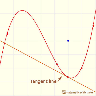
To find the derivative at a point we can draw the tangent line to the graph of a cubic function at that point:
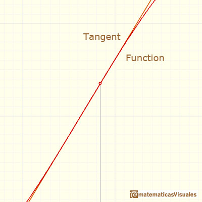
But how can we draw a tangent line?. We can use a magnifying glass!. If we look very near the point in the graph of the function we can see how the function resembles the tangent line. This tangent line
is the best linear approximation of the function at that point:
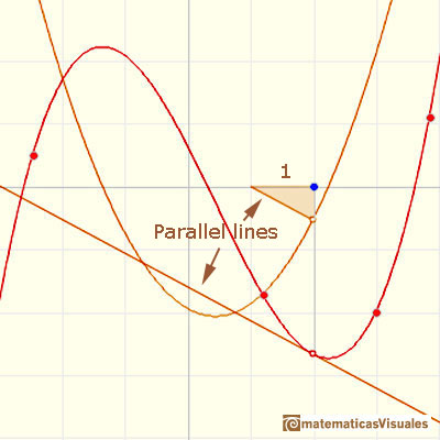
Then we can draw a parallel line to this tangent line through the value x-1 and we get a right triangle:
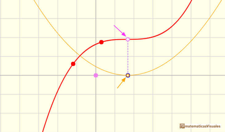
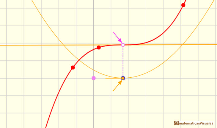
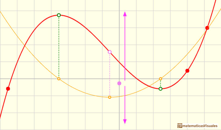
The derivative of a cubic function is a quadratic function.
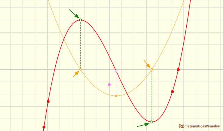
A critical point is a point where the tangent is
parallel to the x-axis, it is to say, that the slope of the
tangent line at that point is zero.
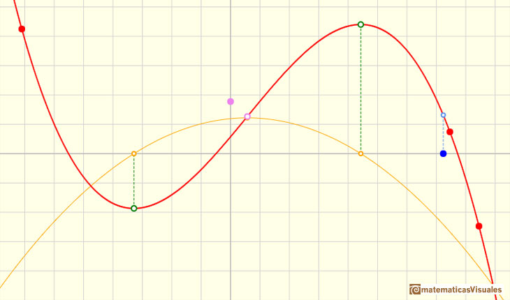
In the following example we can see a cubic function with two critical points. One is a local maximum and the other is
a local minimum. In these points, the derivative function (a parabola) cut the x-axis:
These critical points are points where the function stops increasing or decreasing (some times they are called
"stationary points"). At these points, the tangent is horizontal.
To find the stationary points we solve the quadratic equation:
In this case, solutions of this equation are:
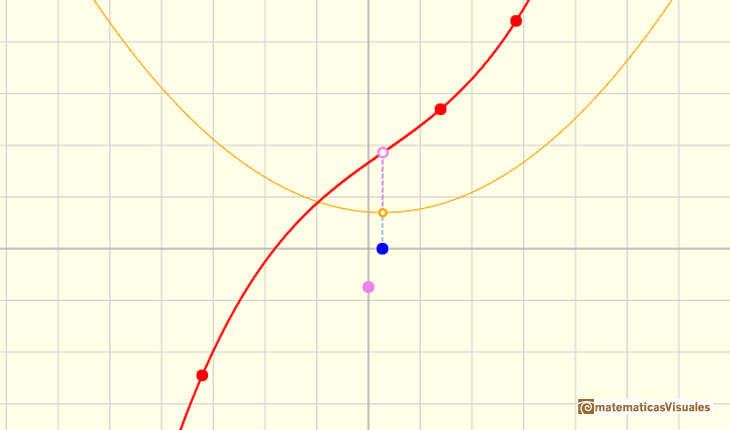
As we already know (quadratic functions), sometimes a quadratic equation has no real solutions.
(the parabola does not cut the x-axis). Then the cubic function has no critical points:
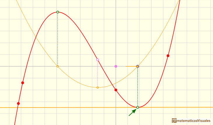
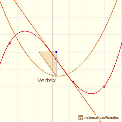
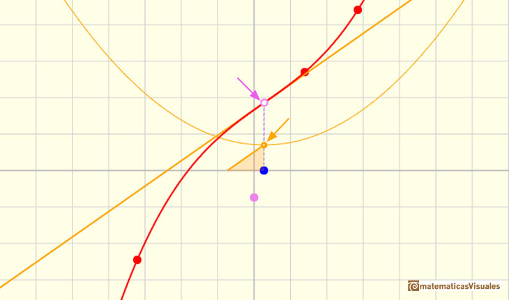
But a parabola has always a vertex. The vertex of the parabola is related with a point of the cubic function. We call
this point an inflection point.
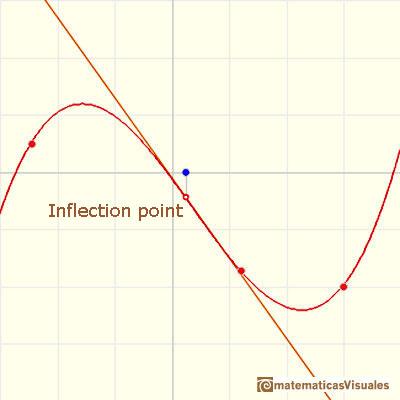
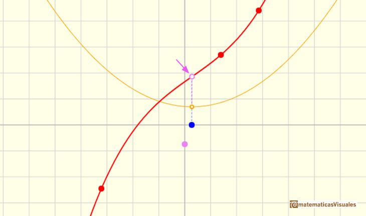
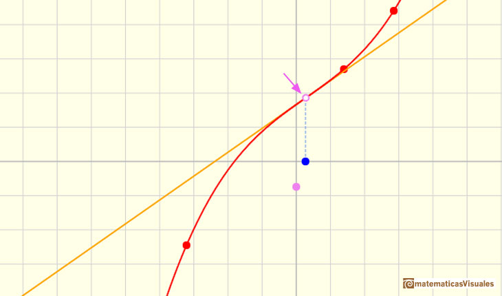
An inflection point of a cubic function is the unique point on the graph where the concavity changes
The curve changes from being concave upwards
to concave downwards, or vice versa
The tangent line of a cubic function at an inflection point crosses the graph:
To find the inflection point we can calculate the vertex of the parabola:
This is an example of an inflection point of a cubic function without critical points:
The inflection point in this case is also an stationary point (the vertex of the derivative touches the x-axis):
Inflection points may be stationary points, but are not local maxima or local minima
One simple and interesting idea is that when we translate up and down the graph of a function (we add or subtract a number from the original function)
the derivative does not change. The reason is very intuitive. When you
move the violet dot you are translating up and down the graph and the derivative is the same:
It is important to notice that the derivative of a polynomial of degree 1 is a constant function (a polynomial of degree 0).
The derivative of a polinomial of degree 2 is a polynomial of degree 1.
And the derivative of a polynomial of degree 3 is a polynomial of degree 2.
When we
derive such a polynomial function the result is a polynomial that has a degree 1 less than the original function.
When we study the integral of a polynomial of degree 2 we can see that in this case the new function is a polynomial of degree 2. One degree more
than the original function. And the integral of a polynomial function is a polynomial function of degree 1 more than the original function.
These results are related to the Fundamental Theorem of Calculus.
REFERENCES
Michael Spivak, Calculus, Third Edition, Publish-or-Perish, Inc.
Tom M. Apostol, Calculus, Second Edition, John Willey and Sons, Inc.
I.M. Gelfand, E.G. Glagoleva, E.E. Shnol, 'Functions and Graphs', Dover Publications, Mineola, N.Y.
 NEXT
NEXT

Lagrange polynomials are polynomials that pases through n given points. We use Lagrange polynomials to explore a general polynomial function and its derivative.
 PREVIOUS

The derivative of a quadratic function is a linear function, it is to say, a straight line.
MORE LINKS

The derivative of a lineal function is a constant function.

If the derivative of F(x) is f(x), then we say that an indefinite integral of f(x) with respect to x is F(x). We also say that F is an antiderivative or a primitive function of f.

Two points determine a stright line. As a function we call it a linear function. We can see the slope of a line and how we can get the equation of a line through two points. We study also the x-intercept and the y-intercept of a linear equation.

Power with natural exponents are simple and important functions. Their inverse functions are power with rational exponents (a radical or a nth root)

Polynomials of degree 2 are quadratic functions. Their graphs are parabolas. To find the x-intercepts we have to solve a quadratic equation. The vertex of a parabola is a maximum of minimum of the function.
Polynomials of degree 3 are cubic functions. A real cubic function always crosses the x-axis at least once.

We can consider the polynomial function that passes through a series of points of the plane. This is an interpolation problem that is solved here using the Lagrange interpolating polynomial.

As an introduction to Piecewise Linear Functions we study linear functions restricted to an open interval: their graphs are like segments.

A piecewise function is a function that is defined by several subfunctions. If each piece is a constant function then the piecewise function is called Piecewise constant function or Step function.

A continuous piecewise linear function is defined by several segments or rays connected, without jumps between them.

The integral concept is associate to the concept of area. We began considering the area limited by the graph of a function and the x-axis between two vertical lines.

Monotonic functions in a closed interval are integrable. In these cases we can bound the error we make when approximating the integral using rectangles.

If we consider the lower limit of integration a as fixed and if we can calculate the integral for different values of the upper limit of integration b then we can define a new function: an indefinite integral of f.

It is easy to calculate the area under a straight line. This is the first example of integration that allows us to understand the idea and to introduce several basic concepts: integral as area, limits of integration, positive and negative areas.

To calculate the area under a parabola is more difficult than to calculate the area under a linear function. We show how to approximate this area using rectangles and that the integral function of a polynomial of degree 2 is a polynomial of degree 3.

We can see some basic concepts about integration applied to a general polynomial function. Integral functions of polynomial functions are polynomial functions with one degree more than the original function.

The Fundamental Theorem of Calculus tell us that every continuous function has an antiderivative and shows how to construct one using the integral.

The Second Fundamental Theorem of Calculus is a powerful tool for evaluating definite integral (if we know an antiderivative of the function).

By increasing the degree, Taylor polynomial approximates the exponential function more and more.

By increasing the degree, Taylor polynomial approximates the sine function more and more.

The function is not defined for values less than -1. Taylor polynomials about the origin approximates the function between -1 and 1.

The function has a singularity at -1. Taylor polynomials about the origin approximates the function between -1 and 1.

The function has a singularity at -1. Taylor polynomials about the origin approximates the function between -1 and 1.

This function has two real singularities at -1 and 1. Taylor polynomials approximate the function in an interval centered at the center of the series. Its radius is the distance to the nearest singularity.

This is a continuos function and has no real singularities. However, the Taylor series approximates the function only in an interval. To understand this behavior we should consider a complex function.

A complex polinomial of degree 3 has three roots or zeros.