After studying some ideas about the integral of lineal functions and quadratic functions,
we can play with the same basic ideas in a more general case.
The focus changed when mathematicians tried to calculate the area under the graph of a function. This lead to the use (and later the definition) of the concept of
integral.
Following Leibniz, we use this symbol to represent the integral:
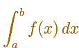
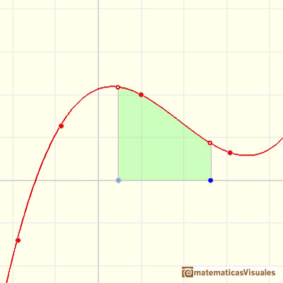
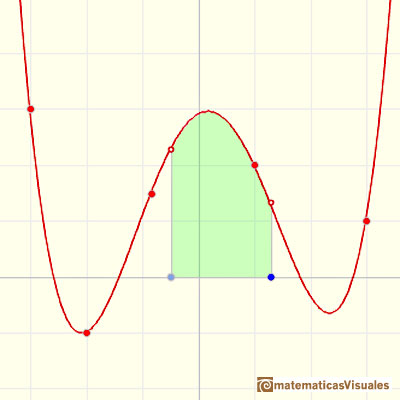
The problem is to calculate the area under the graph of a polynomial function.
One example, with a polynomial function of degree 3:
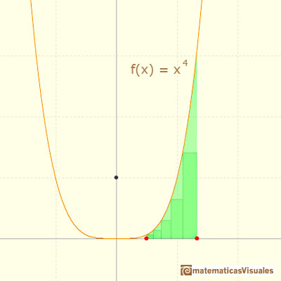
Another example, with a polynomial function of degree 4:
Another example, with a polynomial function of degree 5:
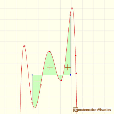
Some areas are positive and some are negative:
The problem for the simple case of polynomial functions was almost solved in Cavalieri's time
(who could calculate the integral for several power
functions).
One important approach is to use rectangles to approximate the area and then take a limit with the bases of these rectangles tend to zero. When
this concept is defined formally this is the Riemann integral.
The integral concept is associate to the concept of area. We began considering the area limited by the graph of a function and the x-axis between two vertical lines.
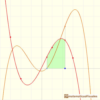
If we consider the lower limit of integration a as fixed and if we can calculate the integral for different values of the upper limit of integration b then we can define a new function: an indefinite integral of f.
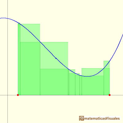
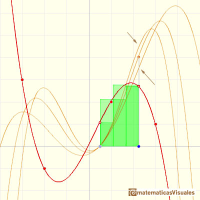
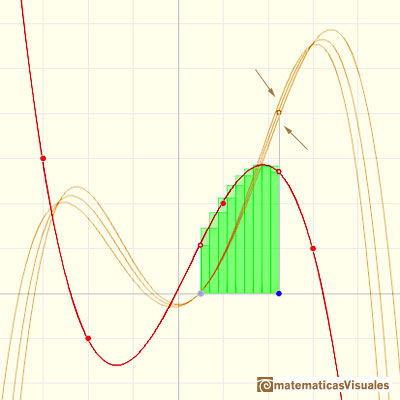
In this intuitive approach we only use rectangles of equal bases. We can see how using rectangles we can approach the area (the function is a polynomial of degree 3, for example, but you can play with different polynomial functions):
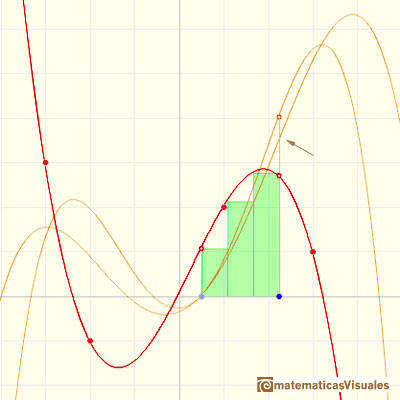
Taking two different values for the height of these rectangles we can get two different approximations:
If we use more and more rectangles the approximations becomes better and better:
It is not always possible to calculate the integral of a function. If we can calculate the indefinite integral of a function we say that this function
is integrable. Polynomial functions are integrable functions.
One integral function of a polynomial of degree n is a polynomial function of degree n+1.
For example, an integral function of a polynomial of degree 3 is a polynomial of degree 4:
If the function is a polynomial of degree 4, an integral function is a polynomial of degree 5:
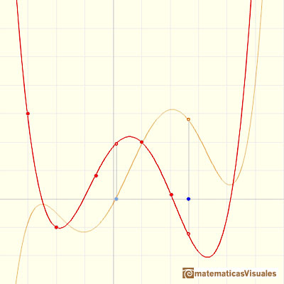
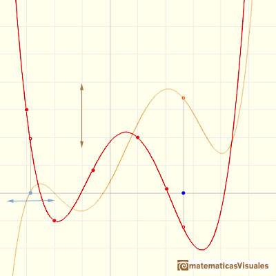
If we change the lower limit of integration, the integral function goes up and down but it does not change its shape. (Why?)
Changing we lower limit of integration we get different integral functions but they are all the same up to a constant (vertical translation).
To calculate the area under a parabola is more difficult than to calculate the area under a linear function. We show how to approximate this area using rectangles and that the integral function of a polynomial of degree 2 is a polynomial of degree 3.
It is easy to calculate the area under a straight line. This is the first example of integration that allows us to understand the idea and to introduce several basic concepts: integral as area, limits of integration, positive and negative areas.
A piecewise function is a function that is defined by several subfunctions. If each piece is a constant function then the piecewise function is called Piecewise constant function or Step function.
The integral concept is associate to the concept of area. We began considering the area limited by the graph of a function and the x-axis between two vertical lines.
Monotonic functions in a closed interval are integrable. In these cases we can bound the error we make when approximating the integral using rectangles.
If we consider the lower limit of integration a as fixed and if we can calculate the integral for different values of the upper limit of integration b then we can define a new function: an indefinite integral of f.
Lagrange polynomials are polynomials that pases through n given points. We use Lagrange polynomials to explore a general polynomial function and its derivative.
If the derivative of F(x) is f(x), then we say that an indefinite integral of f(x) with respect to x is F(x). We also say that F is an antiderivative or a primitive function of f.
Two points determine a stright line. As a function we call it a linear function. We can see the slope of a line and how we can get the equation of a line through two points. We study also the x-intercept and the y-intercept of a linear equation.
Polynomials of degree 2 are quadratic functions. Their graphs are parabolas. To find the x-intercepts we have to solve a quadratic equation. The vertex of a parabola is a maximum of minimum of the function.
We can consider the polynomial function that passes through a series of points of the plane. This is an interpolation problem that is solved here using the Lagrange interpolating polynomial.
In his book 'On Conoids and Spheroids', Archimedes calculated the area of an ellipse. It si a good example of a rigorous proof using a double reductio ad absurdum.


 NEXT
NEXT

 PREVIOUS


