The basic power functions are

n is called the exponent. We start studying power functions with positive integer exponent. The expression xⁿ is known as 'x to the nth power'.

This family includes lines, parabolas, cubic parabolas, etc.

They are the basis of the polynomials.

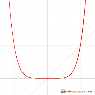
They are examples of even and odd functions. The y-axis of an even function is a symmetry axis for the function: one half of the graph is a 'mirror image' of the other half. When the exponent is even, the function is even:

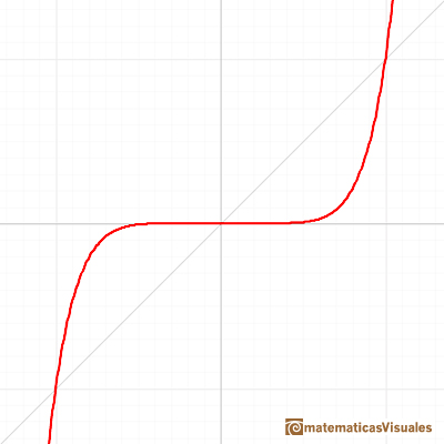
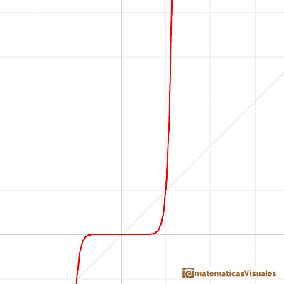
Some functions are symmetric with respect to the origin. These functions are called odd functions. When the exponent of a power functions is odd, the function is odd:

Even and odd power functions have a different end behavior (to the right and to the left).

Seeing this applet we can (intuitively) accept these limits:

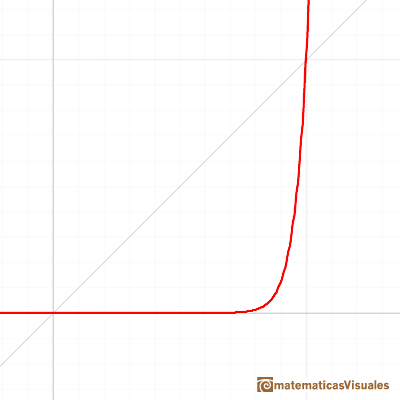
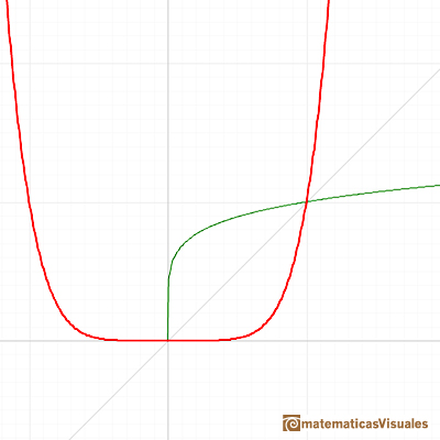
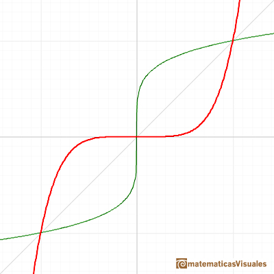
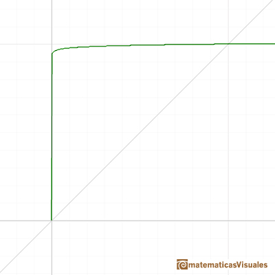
The inverse of exponentiation is extracting a root (the nth root functions):

Root functions are power functions with exponent the reciprocal of a positive integer (n is called the root index).

One function and its inversa are simmetrical respect the first quadrant diagonal. You get the graph of the inverse function reflecting the graph across the line y=x .

The domain of these functions is all the real numbers when n is odd and only the non-negative real numbers when n is even.

Playing with the mathlet you can accept (intuitively) this limit:

MORE LINKS

Polynomial Functions (3): Cubic functions

Polynomials of degree 3 are cubic functions. A real cubic function always crosses the x-axis at least once.

Polynomial Functions (4): Lagrange interpolating polynomial

We can consider the polynomial function that passes through a series of points of the plane. This is an interpolation problem that is solved here using the Lagrange interpolating polynomial.

Polynomial functions and derivative (1): Linear functions

The derivative of a lineal function is a constant function.

Polynomial functions and derivative (2): Quadratic functions

The derivative of a quadratic function is a linear function, it is to say, a straight line.

Polynomial functions and derivative (3): Cubic functions

The derivative of a cubic function is a quadratic function, a parabola.

Polynomial functions and derivative (4): Lagrange polynomials (General polynomial functions)

Lagrange polynomials are polynomials that pases through n given points. We use Lagrange polynomials to explore a general polynomial function and its derivative.

Polynomial functions and derivative (5): Antidifferentiation

If the derivative of F(x) is f(x), then we say that an indefinite integral of f(x) with respect to x is F(x). We also say that F is an antiderivative or a primitive function of f.

Definite integral

The integral concept is associate to the concept of area. We began considering the area limited by the graph of a function and the x-axis between two vertical lines.

Monotonic functions are integrable

Monotonic functions in a closed interval are integrable. In these cases we can bound the error we make when approximating the integral using rectangles.

Indefinite integral

If we consider the lower limit of integration a as fixed and if we can calculate the integral for different values of the upper limit of integration b then we can define a new function: an indefinite integral of f.

Polynomial functions and integral (1): Linear functions

It is easy to calculate the area under a straight line. This is the first example of integration that allows us to understand the idea and to introduce several basic concepts: integral as area, limits of integration, positive and negative areas.

Polynomial functions and integral (2): Quadratic functions

To calculate the area under a parabola is more difficult than to calculate the area under a linear function. We show how to approximate this area using rectangles and that the integral function of a polynomial of degree 2 is a polynomial of degree 3.

Polynomial functions and integral (3): Lagrange polynomials (General polynomial functions)

We can see some basic concepts about integration applied to a general polynomial function. Integral functions of polynomial functions are polynomial functions with one degree more than the original function.

The Fundamental Theorem of Calculus (1)

The Fundamental Theorem of Calculus tell us that every continuous function has an antiderivative and shows how to construct one using the integral.

The Fundamental Theorem of Calculus (2)

The Second Fundamental Theorem of Calculus is a powerful tool for evaluating definite integral (if we know an antiderivative of the function).

Piecewise Linear Functions. Only one piece

As an introduction to Piecewise Linear Functions we study linear functions restricted to an open interval: their graphs are like segments.

Piecewise Constant Functions

A piecewise function is a function that is defined by several subfunctions. If each piece is a constant function then the piecewise function is called Piecewise constant function or Step function.

Continuous Piecewise Linear Functions

A continuous piecewise linear function is defined by several segments or rays connected, without jumps between them.

Complex Polynomial Functions(1): Powers with natural exponent

Complex power functions with natural exponent have a zero (or root) of multiplicity n in the origin.

Complex Polynomial Functions(2): Polynomial of degree 2

A polynomial of degree 2 has two zeros or roots. In this representation you can see Cassini ovals and a lemniscate.

Complex Polynomial Functions(3): Polynomial of degree 3

A complex polinomial of degree 3 has three roots or zeros.

Complex Polynomial Functions(4): Polynomial of degree n

Every complex polynomial of degree n has n zeros or roots.