
|
|

|

|


The integral concept is associated to the concept of area. When a plane figure is bounded by straight lines it is easy to calculate its area. However, areas bounded by curved lines are more difficult to find (and even to define).
One of the key moments of the History of Mathematics was when Archimedes was able to calculate the area of segments of a parabola using Eudoxus' method of exhaustion.
Cavalieri (about 1630) knew how to integrate power functions (f(x)= x^n) from n=1 to as far as n=9. The general result, for arbitrary n, was obtained by Fermat.
Although Cavalieri did not know the term 'function' we can say that one of his contributions was that he considered the problem of calculate the area limited by the graph of a positive function, the x-axis and two vertical lines (a 'curvilinear trapezoid', or 'area under a curve'):
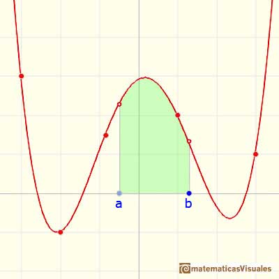
We want to assign a number to this region that represent its area when the function is positive. We are going to call this number the definite integral of f between a and b.
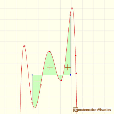
This integral does not always represents the area of a 'curvilinear trapezoid'. This is only the case when f is non-negative. When f is negative the integral is going to be minus the area. In general, the integral is the area of the curvilinear trapezoid that lies above the x-axis diminished by the area of the parts that lie below the x-axis.
If we want to integrate linear functions the problem is simple.
The problem is more difficult when the graph of the function is not a line.
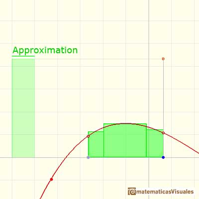
"We shall follow an idea of Archimedes. It is to approximate the function f by horizontal (constant) functions, and the area under f by the sum of little rectangles" (Lang)
In these cases we want to construct the definite integral (a number) as the result of some kind of limiting process. We can start dividing [a,b] into subintervals and take the sum of the areas of certain rectangles which approximate the function f at various points of the interval. The area of these rectangles approximate the integral. Integration is a process of summation.
This is the notation we use:
The symbol S (an elongated S, for sum) is called an integral sign, and it was introduced by Leibniz in 1675. The process which produces the result is called integration. The numbers a and b which are attached to the integral sign are called the lower and upper limits of integration.
Leibniz used this symbol because he considered the integral to be the sum of infinitely many rectangles with height f(x) and "infinitesimal small" width. It was readily accepted by many early mathematicians because they liked to think of integration as a kind of "summation process" which enabled them to add together infinitely many "infinitesimally small quantities".
We are going to try to show some ideas behind the rigurous definition of integral given by Bernhard Riemann (1826-1866).
P is a partition of [a,b].

A partition defines some subintervals. The width of these subintervals could be different:
Given a partition of [a,b] we can add more numbers to the partition and then we get a new partition having small intervals. If we add enough intermediate numbers then the intervals can be made arbitraryly small.
One restriction is the use of regular subdivisions of the interval. In this case the bases of the rectangles are equal:
For each i we choose some point xi* in [xi, xi+1]. The value f(xi*) can be viewed as the height of a rectangle.
"The main idea which we are going to carry out is that, as we make the intervals of our partition smaller and smaller, the sum of the areas of the rectangles will approach a limit, and this limit can be used to define the area under the curve." (Lang)
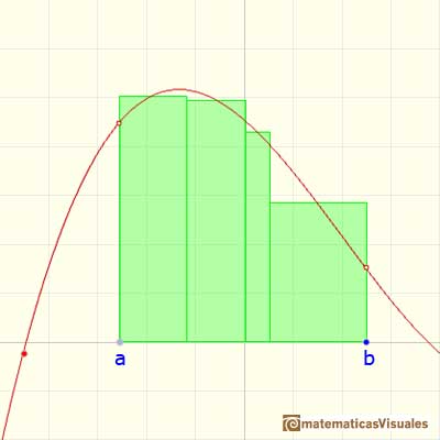
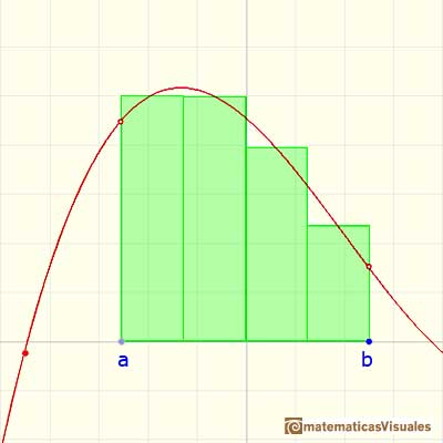
We can choose that xi* to be the point in the middle of the subinterval (as in the mathlet and in the previous examples).
One popular choose is xi* to be equal to xi, the left end of the subinterval. Then the height of the rectangle will be f(xi):
Or we can choose xi* to be equal to xi+1, the right end of the subinterval. Then the height of the rectangle will be f(xi+1):
The election of these xi* in [xi, xi+1] is arbitrary. Then Riemann considered
Any of these sums is called Riemann sum of f for P.
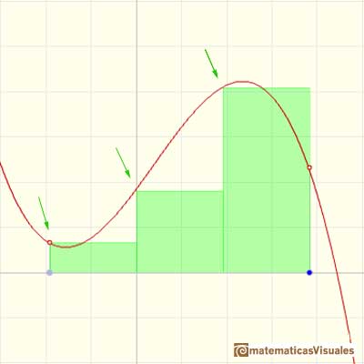
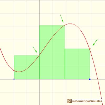
Geometric interpretation: "It is the total area of n rectangles that lies partly below the graph of f and partly above it. Because of the arbitrary way in which the heights of the rectangles have been picked, we can't say for sure whether a particular Riemann sum is less or greater than the integral. But it does seem that the overlap shouldn't matter too much; if the bases of all the rectangles are narrow enough, then the Riemann sum ought to be close to the integral." (Spivak)
If we increase the number of rectangles we (intuitively) will be sometimes closer to a value that is the definite integral.
Then we can say that the definite integral is the limit of the Riemann sums as the number of subdivisions tends to infinity and the width of each subinterval tends to zero. And it does not matter which point xi* we choose in each subinterval.
"The moral of this tale is that anything which looks like a good approximation to an integral really is, provided that all the lengths of the intervals in the partition are small enough." (Spivak)
In the mathlet we can modify the function and the number of rectangles. Although in each interval, the height of the rectangle can be any value of the function in a point of the subinterval, here we consider only one simple possibility: xi* is the middle point of the subinterval. In this case, Riemann sums are called middle Riemann sums.
"The integrals of most functions are impossible to determine exactly (although they may be computed to any degree of accuracy desired by calculating lower and upper sums). Nevertheless, [as we are going to learn later, for example, when we study the Fundamental Theorem of Calculus], the integral of many functions can be computed very easily." (Spivak)
An axiomatic approach to the integral (Following Serge Lang)
In his book 'A First Course in Calculus', before explaining Riemann Sums, he stresses the importance of two properties that will define an integral for f on [a,b]:
Let a, b be two numbers, with a < b. Let f be a continuous function on the interval [a,b]. Suppose that for each pair of number c <=d in the interval we are able to associate a number denoted by

satisfying the following properties:
Property 1. If M, m are two numbers such that
for all x in the interval [c,d] then
Property 2. We have (Additivity)
He also define
After that, he proves that there exists a way of assigning these numbers and that any such assignment is uniquely determined. It is usually denoted by
REFERENCES
 NEXT
NEXT

 PREVIOUS

MORE LINKS


