
|
|

|

|


We are going to study a simple kind of functions. These are Piecewise constant functions or Step functions.
Although these functions are simple they are very important: we use them to approximate other more complex functions and they can help us to get an understanding of the Fundamental Theorem of Calculus from a basic point of view. For example, see Tom Apostol's book.
Some of the ideas and examples of this page are taken from two interesting articles by Gilbert Strang and Antony J. Macula.
A piecewise function is a function that is defined by several subfunctions. Each subfunction apply in a subdomain of the function's domain. In these pages, these subdomains will be intervals. We can say that these functions 'behave differently' based on the input value. For example, we use a different formula depending the input value.
If each piece is a constant function then the piecewise function is called Piecewise constant function or Step function.
For example, the following function has two parts:
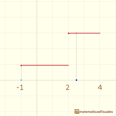
This is a typical notation we use for this function:
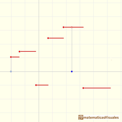
The graph of an step function is made by horizontal segments (or perhaps, rays)
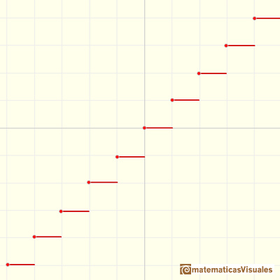
The Floor Function is an example of step function that has an infinite number of pieces.
We remember that the function defined by f(x)=c, where c is a constant, a fixed number, is called a constant function. The graph of a constant function is a horizontal line.
A constant function is a special case of a linear or afine function. The derivative of a linear function is a basic example of derivative, it is a constant function.

The definite integral of a constant function is the area of a rectangle (positive or negative).
The indefinite integral of a constant function is a linear function.

Primitives of a constant function are linear functions.
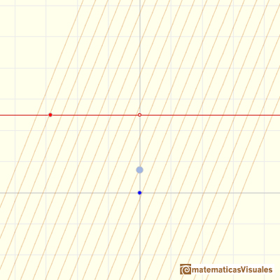
Slopes or these linear functions are the constant function.
Tom Apostol, in his book 'Calculus', began writing about the integral of a function defining the integral of steps functions.
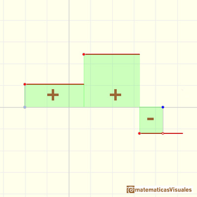
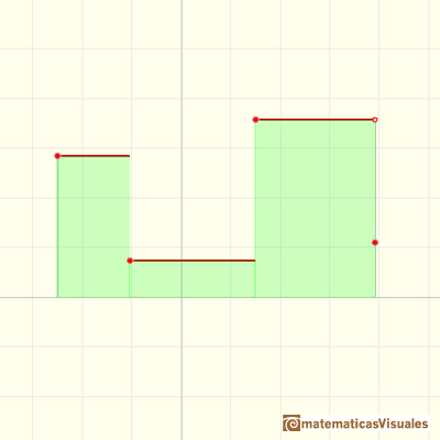
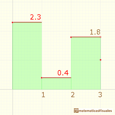
To compute the integral of a step function
we multiply each constant value by the length of the corresponding subinterval.
Then the value of the integral is the sum of the areas (positive or negative) of the individual rectangles. Notice that this value is independent of the values of the step function at the subdivision points. (Apostol, p. 65).
(After that, Apostol prove several important properties of the integral, pags 68-69, and uses this definition to define the integral of more general functions, approximating a function from above and below by step functions. He wrote: "The approach will be patterned somewhat after the method of Archimedes. The idea is simply this: We begin by approximating the function f from below and from above by step functions." (p. 72))
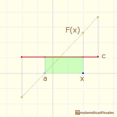
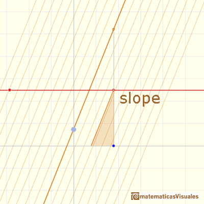
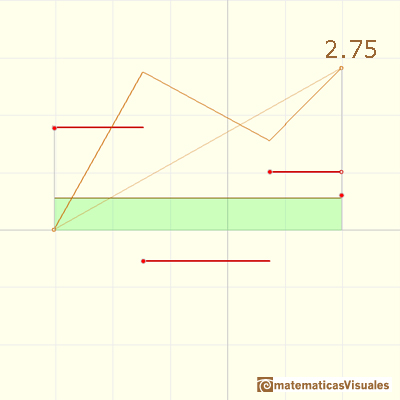
We denote the indefinite integral as the function F(x):
In those intervals where f is constant, the function F is linear. We describe this by saying that the integral of a step function is piecewise linear.(Apostol, p. 123)
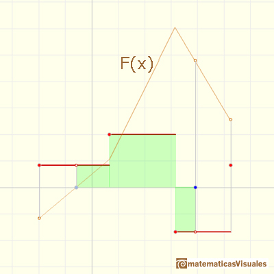
Observe also that the graph of f is made up of disconnected line segments. There are points on the graph of f where a small change in x produces a sudden jump in the value of the function. Note, however, that the corresponding indefinite integral does not exhibit this behavior. A small change in x produces only a small change in F(x). That is why the graph of F is not disconnected. This illustrates a general property of indefinite integrals known as continuity. (Apostol, p. 124).
As Spivak wrote, it appears that F is always better behaved than f.
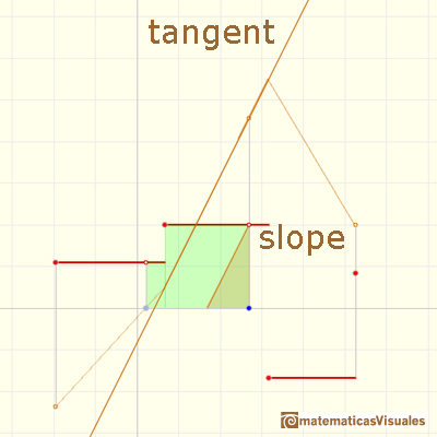
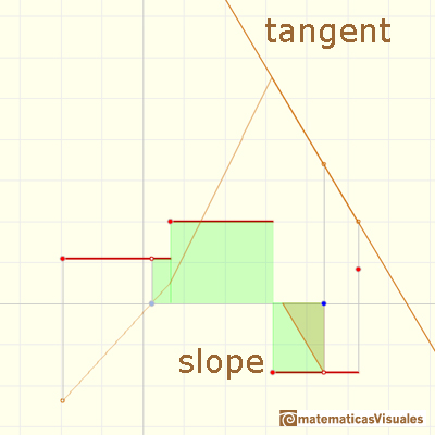
It is interesting to understand the relation between these functions, F and f, that come in pairs. F is the integral of f and f is the derivative of F.
The use of graphs and the ideas of slope and area are tremendous visual supports. In Gilbert Strang's opinion the best approach is see f as velocity and F as distance.
We already know the first pair of functions: constant f and linear F. The second pair is what we are studying now: a piecewise constant f and a piecewise linear F.
Some examples from Gilbert Strang's article (you can try to reproduce these examples using the applet).
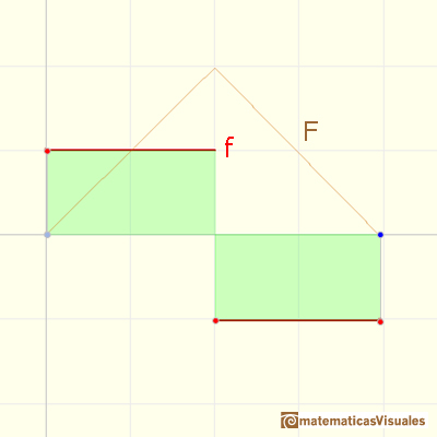
We can see the following graph as going forward and back (positive and negative constant velocity):
A steadily increasing velocity imitates f(x) = 2x
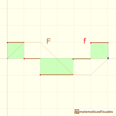
An oscillating velocity imitates f(x) = cos(x) and F(x) resembles roughly a sine curve:
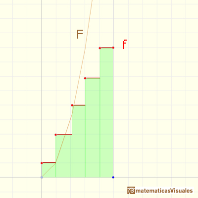
An exponentially increasing velocity imitates f(x) = 2^x:
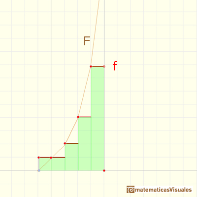
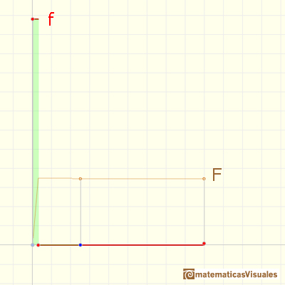
A burst of speed (then stop) makes F imitate a step function:
We see that if f is a step function, F is a continuos piecewise linear function. But this function F is not a differentiable function. At some points it is not 'smooth'. The indefinite integral of a step function is piecewise differentiable.
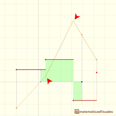
In this case we can say that the piecewise differentiable function F has lateral derivatives but they are not equal at some points:
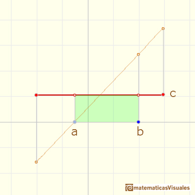
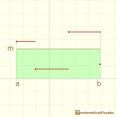
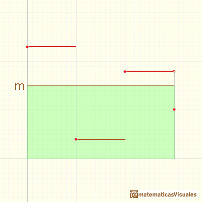
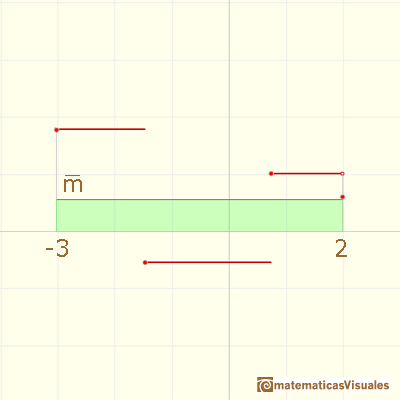
The average value of a function f(x) over the interval [a,b] is given by
You can see the integral as an area or a distance.
One idea is that the area under the function (positive or negative) ...
... is the same as the area of a rectangle whose height is the average value.
First example (simple average):
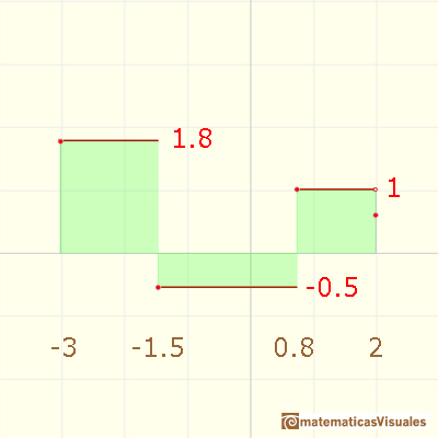
Second example (weighted average):
Next we are going to study more about Continuous Linear Piecewise Functions and their relations with Step Functions and the Fundamental Theorem of Calculus.
REFERENCES
 NEXT
NEXT

 PREVIOUS

MORE LINKS


