matematicas visuales visual math
Antiderivative


There is one important type of problems in which we know the derivative of a function (its rate of change, the slope of its graph) and we want to find the function. For example, we know velocity and want to calculate the space.

The process of finding a function from its derivative is called antidifferentiation, finding a primitive function, or finding an indefinite integral. As the name implies, antidifferentiation is an inverse operation to differentiation.

The use of the word integration here could seem odd because the problem of integration is related in some way with the finding of an area (accumulation, summation) and differentiation is related with the instantaneous rate of change or as the slope of the tangent line to the graph of the function. We are going to see later then this two very different problems are deeply connected (Fundamental Theorem of Calculus) and that, in some way, integration is the inverse process of differentiation.

F(x) is said to be an antiderivative (or a primitive or an indefinite integral) of f(x) on an open interval if the derivative of F is f for every value of x on the interval.

Antiderivative, antidifferentiation, primitive, integral: definition | matematicasVisuales

Notice that we define an antiderivative and not the antiderivative. This is because an antiderivative is not unique. Nevertheless the antiderivative is unique up to an additive constant. It is say:

Any two antiderivatives F and G of the same function f can differ only by a constant.

The reason is because their difference F-G has the derivative 0 and then F-G is a constant function.

Sometimes we use a particular sign (from Leibniz, the sign for integration is a large 's' from 'sum'. Leibniz used the following sign to denote a general primitive of f):

Antiderivative, antidifferentiation, primitive, integral: integral sign, Leibniz | matematicasVisuales

The function f is called the integrand, the constant C is called the constant of integration. The symbol dx indicates that we are to integrate with respect to x.

If we know simple techniques of differentiation to find some antiderivatives is easy. For example, it is straightforward to find a primitive for a constant function:

Antiderivative, antidifferentiation, primitive, integral: primitive of a constant function is a linear function | matematicasVisuales

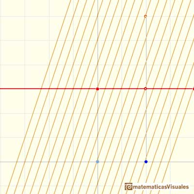
We can check that in each point the derivative is the original constant function:

Antiderivative, antidifferentiation, primitive, integral: checking a primitive of a constant function | matematicasVisuales

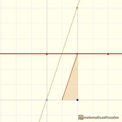
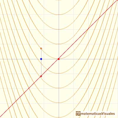
The derivative of a polynomial of degree 1 (linear function) is a constant function (degree 0, an horizontal line). Then, an antiderivative of a constant function is a linear function.

Antiderivatives of polynomials functions are easy too. For example, a basic linear function (the identity function):

Antiderivative, antidifferentiation, primitive, integral: primitive of a linear function is a parabola | matematicasVisuales

Checking the result in one point:

Antiderivative, antidifferentiation, primitive, integral: checking a primitive of a linear function | matematicasVisuales

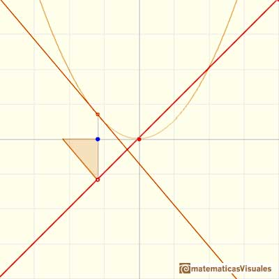
The derivative of a polynomial of degree 2 (a parabola) is a polynomial of degree 1 (a linear function). Then, a primitive of linear function is a parabola.

A quadratic polynomial (a parabola):

Antiderivative, antidifferentiation, primitive, integral: primitive of a parabola is a cubic function | matematicasVisuales
Antiderivative, antidifferentiation, primitive, integral: checking a primitive of a parabola | matematicasVisuales

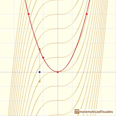
The derivative of a polynomial of degree 3 (a cubic) is a polynomial of degree 2 (a parabola). Then, an antiderivative of a parabola is a cubic function.

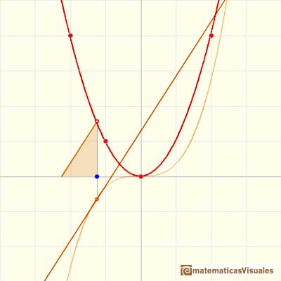
Another example, a cubic polynomial:

Antiderivative, antidifferentiation, primitive, integral: primitive of a cubic function | matematicasVisuales

Antiderivative, antidifferentiation, primitive, integral: checking a primitive of a cubic function | matematicasVisuales

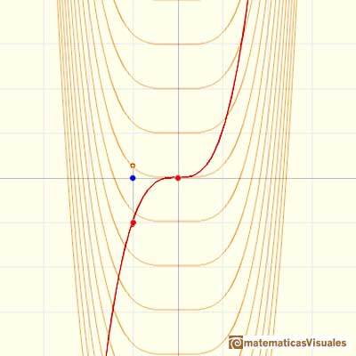
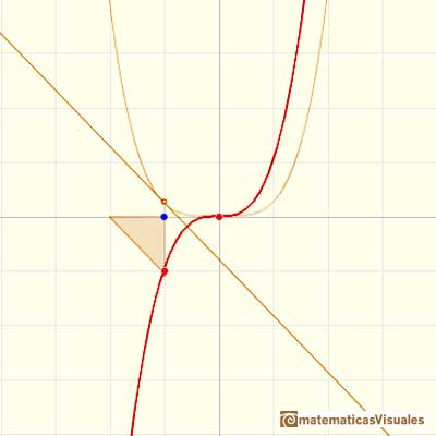
In the next version of the interactive application you can move the blue dot along the x-axis:

When we differentiate a polynomial function we get a polynomial function of one degree less than the original function. When we find an antiderivative of a polynomial function we get a polynomial function of one degree more than the original function.

Although finding primitives of polynomial functions is easy, to find an antiderivative turns out to be a difficult problem in general. The Fundamental Theorem of Calculus tell us that we can always construct an antiderivative (primitive) of a continuous function by integration.

REFERENCES

Michael Spivak, Calculus, Third Edition, Publish-or-Perish, Inc.
Tom M. Apostol, Calculus, Second Edition, John Willey and Sons, Inc.

MORE LINKS

Polynomial functions and derivative (1): Linear functions
The derivative of a lineal function is a constant function.
Polynomial functions and derivative (2): Quadratic functions
The derivative of a quadratic function is a linear function, it is to say, a straight line.
Polynomial functions and derivative (3): Cubic functions
The derivative of a cubic function is a quadratic function, a parabola.
Definite integral
The integral concept is associate to the concept of area. We began considering the area limited by the graph of a function and the x-axis between two vertical lines.
Monotonic functions are integrable
Monotonic functions in a closed interval are integrable. In these cases we can bound the error we make when approximating the integral using rectangles.
Indefinite integral
If we consider the lower limit of integration a as fixed and if we can calculate the integral for different values of the upper limit of integration b then we can define a new function: an indefinite integral of f.
Polynomial functions and integral (2): Quadratic functions
To calculate the area under a parabola is more difficult than to calculate the area under a linear function. We show how to approximate this area using rectangles and that the integral function of a polynomial of degree 2 is a polynomial of degree 3.
Polynomial functions and integral (3): Lagrange polynomials (General polynomial functions)
We can see some basic concepts about integration applied to a general polynomial function. Integral functions of polynomial functions are polynomial functions with one degree more than the original function.
The Fundamental Theorem of Calculus (1)
The Fundamental Theorem of Calculus tell us that every continuous function has an antiderivative and shows how to construct one using the integral.
The Fundamental Theorem of Calculus (2)
The Second Fundamental Theorem of Calculus is a powerful tool for evaluating definite integral (if we know an antiderivative of the function).
Piecewise Linear Functions. Only one piece
As an introduction to Piecewise Linear Functions we study linear functions restricted to an open interval: their graphs are like segments.
Piecewise Constant Functions
A piecewise function is a function that is defined by several subfunctions. If each piece is a constant function then the piecewise function is called Piecewise constant function or Step function.
Continuous Piecewise Linear Functions
A continuous piecewise linear function is defined by several segments or rays connected, without jumps between them.
Integral of powers with natural exponent
The integral of power functions was know by Cavalieri from n=1 to n=9. Fermat was able to solve this problem using geometric progressions.
Polynomial Functions (1): Linear functions
Two points determine a stright line. As a function we call it a linear function. We can see the slope of a line and how we can get the equation of a line through two points. We study also the x-intercept and the y-intercept of a linear equation.
Powers with natural exponents (and positive rational exponents)
Power with natural exponents are simple and important functions. Their inverse functions are power with rational exponents (a radical or a nth root)
Polynomial Functions (2): Quadratic functions
Polynomials of degree 2 are quadratic functions. Their graphs are parabolas. To find the x-intercepts we have to solve a quadratic equation. The vertex of a parabola is a maximum of minimum of the function.
Polynomial Functions (3): Cubic functions
Polynomials of degree 3 are cubic functions. A real cubic function always crosses the x-axis at least once.
Polynomial Functions (4): Lagrange interpolating polynomial
We can consider the polynomial function that passes through a series of points of the plane. This is an interpolation problem that is solved here using the Lagrange interpolating polynomial.
Taylor polynomials (1): Exponential function
By increasing the degree, Taylor polynomial approximates the exponential function more and more.
Taylor polynomials (2): Sine function
By increasing the degree, Taylor polynomial approximates the sine function more and more.