Given a function and two real values, a and b (these two numbers are called limits of integration), we write the definite integral as
The intuitive meaning is the area bounded between the x-axis, the graph of the function and the vertical lines x = a and x = b. In some cases that area is considered
positive and in other cases is negative. We are going to see some examples later.
The integral concept is associate to the concept of area. We began considering the area limited by the graph of a function and the x-axis between two vertical lines.
If we consider the lower limit of integration a as fixed and if we can calculate the integral for different values of the upper limit of integration b then we can define a new function: an indefinite integral of f.
The objective of this page is to play with these ideas in the simplest case of linear functions.
A linear function is a polynomial of degree equal or less than 1 and its graph is a straight line.
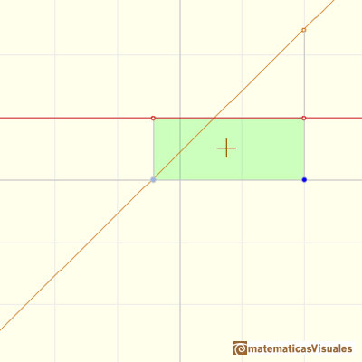
We can start with constant functions (horizontal lines). We can consider constant functions as polynomial functions of degree 0.
In this case the area is above the x-axis, then the area (the integral) is positive.
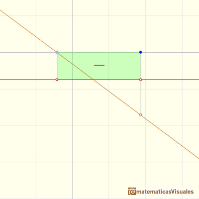
In this case the area is below the x-axis, then the area (the integral) is negative.
The integral of a constant function (a polynomial of degree 0) is a straight line, it is to say, a polynomial of degree 1. (The constant function
f(x) = 0 is an exception).
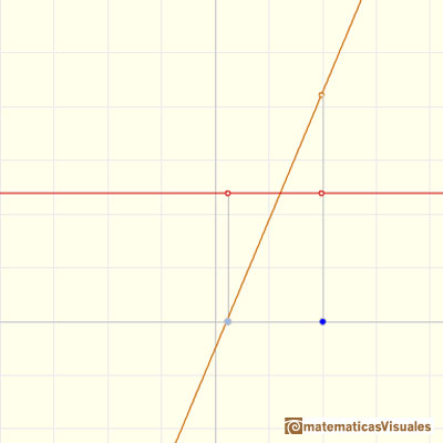
If we change the constant function you can see that the integral changes. But the only thing that change is the slope of the line.
If we change the "lower" limit of integration (blue pale dot) we can see how the straight line is going up and down.
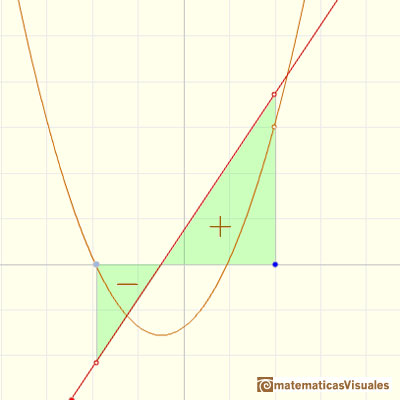
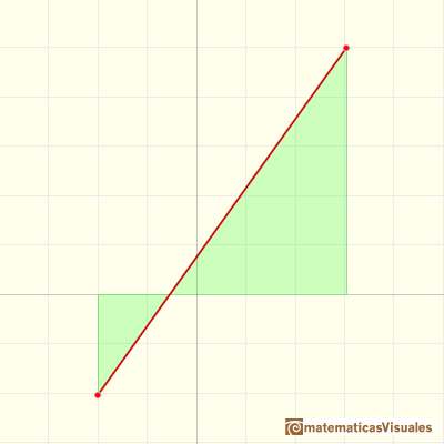
When we consider a general linear function it is still very easy to calculate the integral function. In these cases we can see that some areas are
positive and some areas are negative:
We say that quadratic functions are integrable functions because we can calculate an indefinite integral of a parabola.
The integral function of a linear function (a polynomial of degree 1) is a parabola (a polynomial of degree 2).
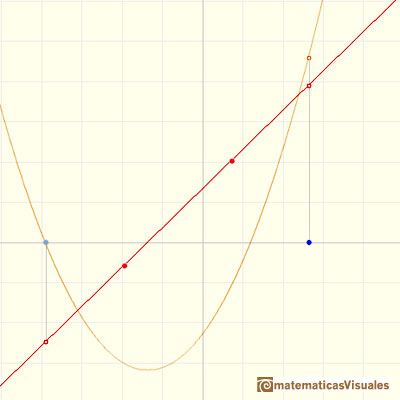
If we change the lower limit of integration, the integral function (the parabola) goes up and down. (Why?)
Changing we lower limit of integration we get different integral functions but they are all the same up to a constant (vertical translation).
The integral function of a constant function (a polynomial of degree 0) is a polynomial of degree 1. The integral function of a polynomial of degree 1 is
a polynomial of degree 2. When we integrate these functions the result is a polynomial of degree one more than the original function.
Remember that when we derive a linear function the result is one less than the original function.
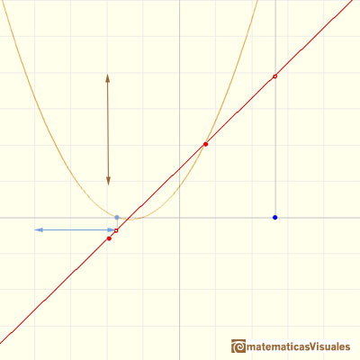
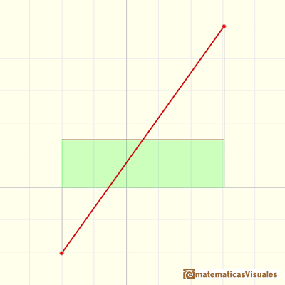
Now we are going to study the average value of a function in this simple case of linear functions.
The average value of a function f(x) over the interval [a,b] is given by
The idea is that the area under the function (positive or negative) ...
... is the same as the area of a rectangle whose height is the average value.
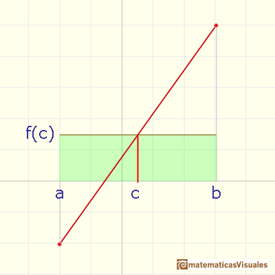
As Linear Function are continuous, they are special cases of the Mean Value Theorem for integrals: If f(x) is a
continuous function over the interval [a,b] then there is a number c in [a,b] such that
REFERENCES
Michael Spivak, Calculus, Third Edition, Publish-or-Perish, Inc.
Tom M. Apostol, Calculus, Second Edition, John Willey and Sons, Inc.
To calculate the area under a parabola is more difficult than to calculate the area under a linear function. We show how to approximate this area using rectangles and that the integral function of a polynomial of degree 2 is a polynomial of degree 3.
If the derivative of F(x) is f(x), then we say that an indefinite integral of f(x) with respect to x is F(x). We also say that F is an antiderivative or a primitive function of f.
We can see some basic concepts about integration applied to a general polynomial function. Integral functions of polynomial functions are polynomial functions with one degree more than the original function.
A piecewise function is a function that is defined by several subfunctions. If each piece is a constant function then the piecewise function is called Piecewise constant function or Step function.
The integral concept is associate to the concept of area. We began considering the area limited by the graph of a function and the x-axis between two vertical lines.
Monotonic functions in a closed interval are integrable. In these cases we can bound the error we make when approximating the integral using rectangles.
If we consider the lower limit of integration a as fixed and if we can calculate the integral for different values of the upper limit of integration b then we can define a new function: an indefinite integral of f.
Lagrange polynomials are polynomials that pases through n given points. We use Lagrange polynomials to explore a general polynomial function and its derivative.
If the derivative of F(x) is f(x), then we say that an indefinite integral of f(x) with respect to x is F(x). We also say that F is an antiderivative or a primitive function of f.
Two points determine a stright line. As a function we call it a linear function. We can see the slope of a line and how we can get the equation of a line through two points. We study also the x-intercept and the y-intercept of a linear equation.
Polynomials of degree 2 are quadratic functions. Their graphs are parabolas. To find the x-intercepts we have to solve a quadratic equation. The vertex of a parabola is a maximum of minimum of the function.
We can consider the polynomial function that passes through a series of points of the plane. This is an interpolation problem that is solved here using the Lagrange interpolating polynomial.
In his book 'On Conoids and Spheroids', Archimedes calculated the area of an ellipse. It si a good example of a rigorous proof using a double reductio ad absurdum.


 NEXT
NEXT

 PREVIOUS


