The first fundamental theorem of calculus tell us that we can always construct a
primitive of a continuous function
by integration. When we combine this with the fact that two primitives of the same function can differ only by a constant, we obtain the Second
Fundamental Theorem of Calculus. (Apostol)
The Second Fundamental Theorem of Calculus (with a weak hypothesis) says: Assume f is continuous on an open interval I,
and let P be any primitive (an indefinite integral, P'=f) of f on I. Then, for each a and each b in I, we have
The demonstration is not difficult:
Let
Then, for the First Theorem of Calculus:
There is a constant C such that
We can evaluate C because
Then C is
We can write
This expression is true for x=b, and our result follows:
This theorem tells us that we can compute the value of a definite integral by a mere subtraction if we know a primitive (antiderivative) F.
The problem of evaluating
an integral is transferred to another problem, that of finding a primitive F of f. Every differentiation formula, when read in reverse,
gives us an example of a primitive of some function
f and this, in turn, leads to an integration formula for this function. (Apostol)
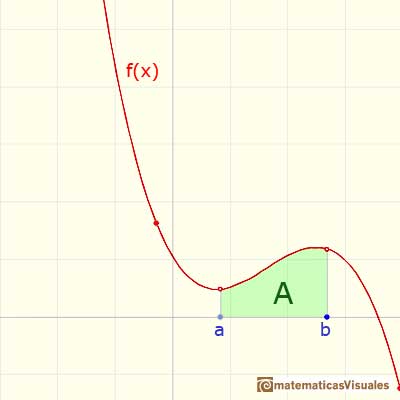
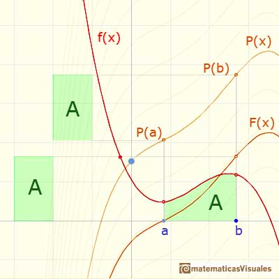
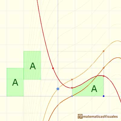
We want to calculate a definite integral of a function f:
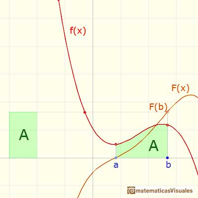
The integral function F is:
If we know how to calculate another primitive or antiderivative P of f we can calculate very easily (only substracting) the value of the integral:
If we choose another antiderivative, the result is the same:
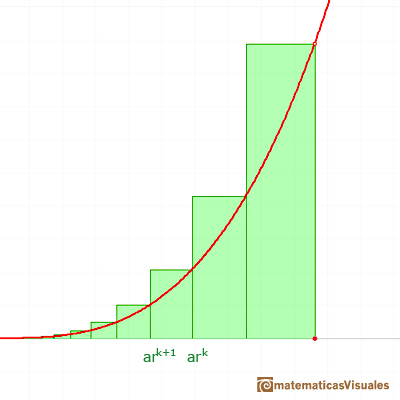
Or the different techniques that Cavalieri, Fermat and others needed
to integrate power functions (1800 years later):
With the powerful tool that this theorem provided us, to integrate this kind of integrals is routine. For example, if we want to integrate
We look for a primitive or antiderivative of the integrand:
And we apply the theorem:
The result is:
And, in general, it is easy to integrate power functions:
The Second Fundamental Theorem of Calculus provides us with a powerful tool for evaluating definite integrals exactly but is useful only when we can fin an antiderivative for
the function being integrated. Sometimes this is a easy task but sometimes it is difficult.
In order to use the theorem in the evaluation of definite integrals we must develop some procedures to aid in finding antiderivatives.
They are called 'Techniques of Integration'.
It is very typical to use the letter F for a primitive or antiderivative of f. And to denote the difference F(b)-F(a), as a short-hand notation, we use the symbol
A basic example:
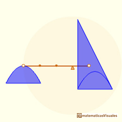
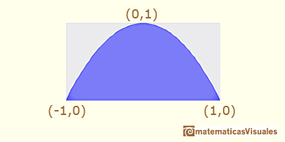
Another basic example: we know that Archimedes was able to calculate the area of a parabolic segment. Now we can use
the Fundamental Theorem of Calculus. We want to calculate this area:
We are going to evaluate the area using the integral:
And the calculation is straightforward:
As I said before, the hypothesis of the Second Fundamental Theorem is stronger because it applies to every integrable function f (not necessarily
continuous). This is a more difficult result to probe.
REFERENCES
Michael Spivak, Calculus, Third Edition, Publish-or-Perish, Inc.
Tom M. Apostol, Calculus, Second Edition, John Willey and Sons, Inc.
Otto Toeplitz, The Calculus, a genetic approach, The University of Chicago Press, 1963 (p. 95-99).
Kenneth A. Ross, Elementary Analysis: The Theory of Calculus, Springer-Verlag New York Inc., 1980 (p. 190).
Serge Lang, A First Course in Calculus, Third Edition, Addison-Wesley Publishing Company.
David M. Bressoud, Historical Reflections on Teaching the Fundamental Theorem of Calculus, American Mathematical Monthly 118 (2011).
If the derivative of F(x) is f(x), then we say that an indefinite integral of f(x) with respect to x is F(x). We also say that F is an antiderivative or a primitive function of f.
It is easy to calculate the area under a straight line. This is the first example of integration that allows us to understand the idea and to introduce several basic concepts: integral as area, limits of integration, positive and negative areas.
To calculate the area under a parabola is more difficult than to calculate the area under a linear function. We show how to approximate this area using rectangles and that the integral function of a polynomial of degree 2 is a polynomial of degree 3.
If the derivative of F(x) is f(x), then we say that an indefinite integral of f(x) with respect to x is F(x). We also say that F is an antiderivative or a primitive function of f.
The integral concept is associate to the concept of area. We began considering the area limited by the graph of a function and the x-axis between two vertical lines.
Monotonic functions in a closed interval are integrable. In these cases we can bound the error we make when approximating the integral using rectangles.
If we consider the lower limit of integration a as fixed and if we can calculate the integral for different values of the upper limit of integration b then we can define a new function: an indefinite integral of f.
A piecewise function is a function that is defined by several subfunctions. If each piece is a constant function then the piecewise function is called Piecewise constant function or Step function.
Lagrange polynomials are polynomials that pases through n given points. We use Lagrange polynomials to explore a general polynomial function and its derivative.
Two points determine a stright line. As a function we call it a linear function. We can see the slope of a line and how we can get the equation of a line through two points. We study also the x-intercept and the y-intercept of a linear equation.
Polynomials of degree 2 are quadratic functions. Their graphs are parabolas. To find the x-intercepts we have to solve a quadratic equation. The vertex of a parabola is a maximum of minimum of the function.
We can consider the polynomial function that passes through a series of points of the plane. This is an interpolation problem that is solved here using the Lagrange interpolating polynomial.
In his book 'On Conoids and Spheroids', Archimedes calculated the area of an ellipse. It si a good example of a rigorous proof using a double reductio ad absurdum.


 PREVIOUS


