We start with a set of n+1 points on the plane with different x-coordinates

(x₀, y₀), (x₁, y₁), (x₂, y₂),....,(x_n, y_n).

Our objective is to find a polynomial function that passes through these n+1 points. A polynomial that passes through several points is called an interpolating polynomial.

One form of the solution is the Lagrange interpolating polynomial (Lagrange published his formula in 1795 but this polynomial was first published by Waring in 1779 and rediscovered by Euler in 1783).

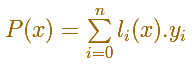
The general formula for the Lagrange interpolating polynomial is

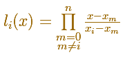
We use Lagrange basis polynomials:

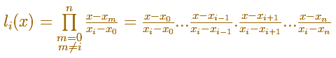
Expanding the product:

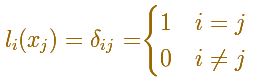
These Lagrange basis polynomials are built to have a property:

Then it is very easy to check that this polynomials passes through all n+1 points given (it is an interpolating polynomial):

The degree of the Lagrange interpolating polynomial is equal or less than n. It has the least degree possible and it is unique.

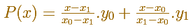
We can see some examples. The simplest one is a straight line. Given two points (x₀, y₀) and (x₁, y₁) there is exactly one line through these two points:

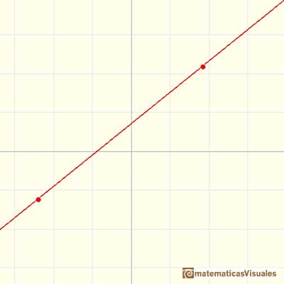
Given three points (x₀, y₀), (x₁, y₁) and (x₂, y₂), with different x-coordinates, either the three points lie in a line or there is a second degree polynomial (a parabola) through these three points. In any case, there is a polynomial of degree at most 2 passing through these three points.

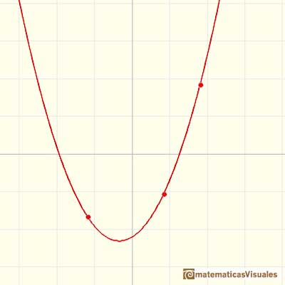
If you have four points, you can find a cubic polynomial (or a parabola, or a straight line in some cases) through them:

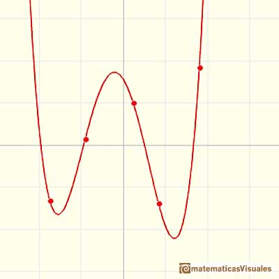
A polynomial function of degree 4 that passes through 5 points:

We are going to use Lagrange polynomials to build interactive applications to play with polynomial functions, their derivatives and integrals.

Polynomial Functions with real or complex coefficients of degree n always have n roots (real or complex) (Fundamental Theorem of Algebra):

MORE LINKS

Polynomial Functions (1): Linear functions

Two points determine a stright line. As a function we call it a linear function. We can see the slope of a line and how we can get the equation of a line through two points. We study also the x-intercept and the y-intercept of a linear equation.

Powers with natural exponents (and positive rational exponents)

Power with natural exponents are simple and important functions. Their inverse functions are power with rational exponents (a radical or a nth root)

Polynomial Functions (2): Quadratic functions

Polynomials of degree 2 are quadratic functions. Their graphs are parabolas. To find the x-intercepts we have to solve a quadratic equation. The vertex of a parabola is a maximum of minimum of the function.

Polynomial functions and derivative (2): Quadratic functions

The derivative of a quadratic function is a linear function, it is to say, a straight line.

Polynomial functions and derivative (3): Cubic functions

The derivative of a cubic function is a quadratic function, a parabola.

Piecewise Linear Functions. Only one piece

As an introduction to Piecewise Linear Functions we study linear functions restricted to an open interval: their graphs are like segments.

Piecewise Constant Functions

A piecewise function is a function that is defined by several subfunctions. If each piece is a constant function then the piecewise function is called Piecewise constant function or Step function.

Continuous Piecewise Linear Functions

A continuous piecewise linear function is defined by several segments or rays connected, without jumps between them.

Rational Functions (1): Linear rational functions

Rational functions can be writen as the quotient of two polynomials. Linear rational functions are the simplest of this kind of functions.

Rational Functions (2): degree 2 denominator

When the denominator of a rational function has degree 2 the function can have two, one or none real singularities.

Polynomial functions and derivative (4): Lagrange polynomials (General polynomial functions)

Lagrange polynomials are polynomials that pases through n given points. We use Lagrange polynomials to explore a general polynomial function and its derivative.

Polynomial functions and derivative (5): Antidifferentiation

If the derivative of F(x) is f(x), then we say that an indefinite integral of f(x) with respect to x is F(x). We also say that F is an antiderivative or a primitive function of f.

Definite integral

The integral concept is associate to the concept of area. We began considering the area limited by the graph of a function and the x-axis between two vertical lines.

Monotonic functions are integrable

Monotonic functions in a closed interval are integrable. In these cases we can bound the error we make when approximating the integral using rectangles.

Indefinite integral

If we consider the lower limit of integration a as fixed and if we can calculate the integral for different values of the upper limit of integration b then we can define a new function: an indefinite integral of f.

Polynomial functions and integral (1): Linear functions

It is easy to calculate the area under a straight line. This is the first example of integration that allows us to understand the idea and to introduce several basic concepts: integral as area, limits of integration, positive and negative areas.

Polynomial functions and integral (2): Quadratic functions

To calculate the area under a parabola is more difficult than to calculate the area under a linear function. We show how to approximate this area using rectangles and that the integral function of a polynomial of degree 2 is a polynomial of degree 3.

Polynomial functions and integral (3): Lagrange polynomials (General polynomial functions)

We can see some basic concepts about integration applied to a general polynomial function. Integral functions of polynomial functions are polynomial functions with one degree more than the original function.

The Fundamental Theorem of Calculus (1)

The Fundamental Theorem of Calculus tell us that every continuous function has an antiderivative and shows how to construct one using the integral.

The Fundamental Theorem of Calculus (2)

The Second Fundamental Theorem of Calculus is a powerful tool for evaluating definite integral (if we know an antiderivative of the function).

Taylor polynomials (1): Exponential function

By increasing the degree, Taylor polynomial approximates the exponential function more and more.

Taylor polynomials (2): Sine function

By increasing the degree, Taylor polynomial approximates the sine function more and more.

Taylor polynomials (3): Square root

The function is not defined for values less than -1. Taylor polynomials about the origin approximates the function between -1 and 1.

Taylor polynomials (4): Rational function 1

The function has a singularity at -1. Taylor polynomials about the origin approximates the function between -1 and 1.

Taylor polynomials (5): Rational function 2

The function has a singularity at -1. Taylor polynomials about the origin approximates the function between -1 and 1.

Taylor polynomials (6): Rational function with two real singularities

This function has two real singularities at -1 and 1. Taylor polynomials approximate the function in an interval centered at the center of the series. Its radius is the distance to the nearest singularity.

Taylor polynomials (7): Rational function without real singularities

This is a continuos function and has no real singularities. However, the Taylor series approximates the function only in an interval. To understand this behavior we should consider a complex function.

Complex Polynomial Functions(1): Powers with natural exponent

Complex power functions with natural exponent have a zero (or root) of multiplicity n in the origin.

Complex Polynomial Functions(2): Polynomial of degree 2

A polynomial of degree 2 has two zeros or roots. In this representation you can see Cassini ovals and a lemniscate.

Complex Polynomial Functions(3): Polynomial of degree 3

A complex polinomial of degree 3 has three roots or zeros.

Complex Polynomial Functions(4): Polynomial of degree n

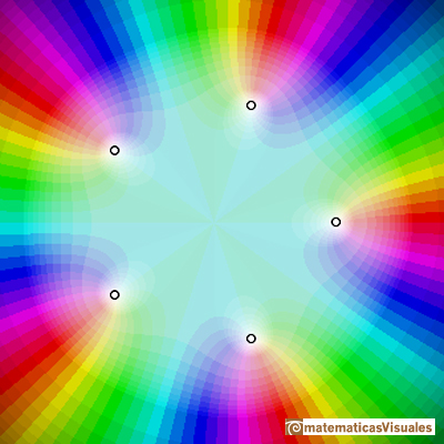
Every complex polynomial of degree n has n zeros or roots.