We have already seen that Real Cubic Functions can have, at most, three real zeros (also called roots).

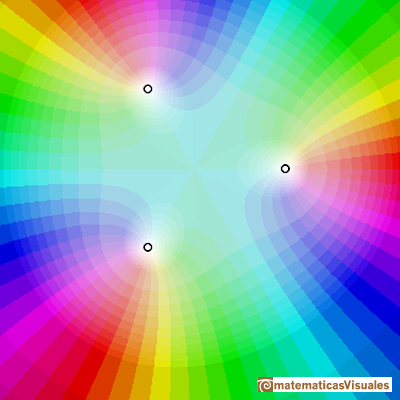
When we consider a cubic function in the complex plane it always have three roots. They are particular cases of polynomial functions. The Fundamental Theorem of Algebra states that every polynomial function of degree n has exactly n complex zeros, not necessarily distinct.

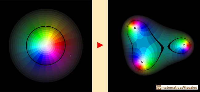
You start the applet seeing the representantion of the cubic polynomial function whose zeros are the cubic roots of unity.

When you change the roots (or zeros) the applet represents a more general cubic function

You can move the dots that represent the different zeros or roots (three simple roots) of the polynomial function. If some of these roots are the same we say that they have double or triple multiplicity.

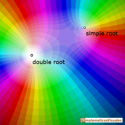
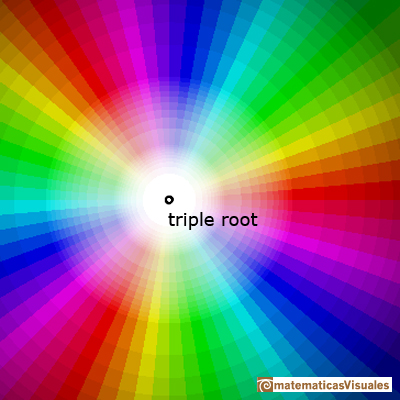
The multiplicity of the zero is represented by the number of times that the color cycle (red->green->blue) goes round the root.

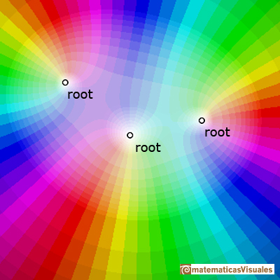
This is another example with three simple roots:

In this example you can see a double root and a simple root:

Round the double root the color cycle repeat itself twice.

This is an example of a triple root:

Round the triple root the color cycle repeat itself three times.

You can see another applet version with darker colors:

In the next applet you can play with a color code that uses a grid (or use the polar color code as before). You can see in black the points that are transformed into complex numbers with module "near" 1.

This is an example using the grid color code:

The same polynomial function using a polar color code:

MORE LINKS

Complex Polynomial Functions(1): Powers with natural exponent Complex power functions with natural exponent have a zero (or root) of multiplicity n in the origin.

Complex Polynomial Functions(5): Polynomial of degree n (variant) Every complex polynomial of degree n has n zeros or roots.

Polynomial Functions (1): Linear functions Two points determine a stright line. As a function we call it a linear function. We can see the slope of a line and how we can get the equation of a line through two points. We study also the x-intercept and the y-intercept of a linear equation.

Polynomial Functions (2): Quadratic functions Polynomials of degree 2 are quadratic functions. Their graphs are parabolas. To find the x-intercepts we have to solve a quadratic equation. The vertex of a parabola is a maximum of minimum of the function.

Polynomial Functions (3): Cubic functions Polynomials of degree 3 are cubic functions. A real cubic function always crosses the x-axis at least once.

Polynomial Functions (4): Lagrange interpolating polynomial We can consider the polynomial function that passes through a series of points of the plane. This is an interpolation problem that is solved here using the Lagrange interpolating polynomial.

Cero and polo (Spanish) Podemos modificar las multiplicidades del cero y del polo de estas funciones sencillas.

Cero and polo (variant) (Spanish)

Moebius transformations (Spanish) Una primera aproximación a estas transformaciones. Representación de dos haces coaxiales de circunferencias ortogonales.

The Complex Exponential Function The Complex Exponential Function extends the Real Exponential Function to the complex plane.

The Complex Cosine Function The Complex Cosine Function extends the Real Cosine Function to the complex plane. It is a periodic function that shares several properties with his real ancestor.

The Complex Cosine Function: mapping an horizontal line The Complex Cosine Function maps horizontal lines to confocal ellipses.

Inversion Inversion is a plane transformation that transform straight lines and circles in straight lines and circles.

Inversion: an anticonformal transformation Inversion preserves the magnitud of angles but the sense is reversed. Orthogonal circles are mapped into orthogonal circles

Multifunctions: Powers with fractional exponent The usual definition of a function is restrictive. We may broaden the definition of a function to allow f(z) to have many differente values for a single value of z. In this case f is called a many-valued function or a multifunction.

Multifunctions: Two branch points Multifunctions can have more than one branch point. In this page we can see a two-valued multifunction with two branch points.

Taylor polynomials: Complex Exponential Function The complex exponential function is periodic. His power series converges everywhere in the complex plane.

Taylor polynomials: Complex Cosine Function The power series of the Cosine Function converges everywhere in the complex plane.

Taylor polynomials: Rational function with two complex singularities We will see how Taylor polynomials approximate the function inside its circle of convergence.