We have already seen that Real Quadratic Functions can have, at most, two real zeros (also called roots).

When we consider a quadratic function in the complex plane it always have two roots. They are particular cases of polynomial functions. The Fundamental Theorem of Algebra states that every polynomial function of degree n has exactly n complex zeros, not necessarily distinct.

In the video we start representing the function

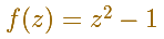
When we transform each point in the complex plane we get a new point. We associate a color to this point. These colors are related to the polar coordinates.

When we move the points, in general, we are seeing a representation of the function:

In this representation, you can see a family of curves that are level curves of the modular surface of the function. Points at the same curve have the property that the product of the distances to the roots of the functions are constant. Then these curves are Cassini Ovals and, between them, the lemniscate.

These ovals where studied by Cassini and he tought that planet trajectories followed this kind of curves. That was before Newton settled the question. These oval where known by the ancient Greek geometer Perseus (around 150 BC) as a toric sections (spiric sections or spiric of Perseus).

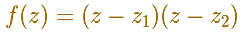
Near a zero you can zoom and see that near a zero the polynomial function is "like a cone" and the level curves are near circles.

You can move the dots that represent two different zeros or roots (two simple roots) of the polynomial function.

If the two roots are the same then we say that it is a double root (a root with multiplicity 2).

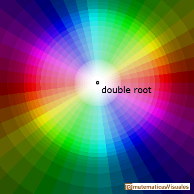
In the case of a double root you can see that the cycle of colors (red, yellow, green, blue) goes round the root twice.

In the next video you can play with a color code that uses a grid (or use the polar color code as before). You can see in black the points that are transformed into complex numbers with module "near" 1.

This is an example using the grid color code:

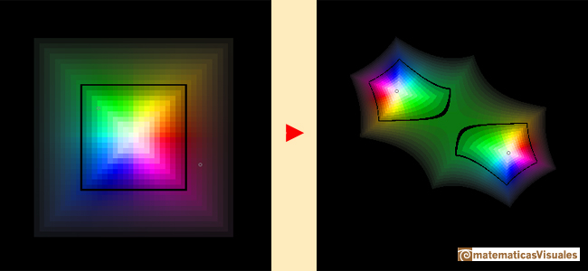
The same polynomial function using a polar color code:

MORE LINKS

Complex Polynomial Functions(4): Polynomial of degree n

Every complex polynomial of degree n has n zeros or roots.

Complex Polynomial Functions(5): Polynomial of degree n (variant)

Every complex polynomial of degree n has n zeros or roots.

Polynomial Functions (1): Linear functions

Two points determine a stright line. As a function we call it a linear function. We can see the slope of a line and how we can get the equation of a line through two points. We study also the x-intercept and the y-intercept of a linear equation.

Polynomial Functions (2): Quadratic functions

Polynomials of degree 2 are quadratic functions. Their graphs are parabolas. To find the x-intercepts we have to solve a quadratic equation. The vertex of a parabola is a maximum of minimum of the function.

Polynomial Functions (3): Cubic functions

Polynomials of degree 3 are cubic functions. A real cubic function always crosses the x-axis at least once.

Polynomial Functions (4): Lagrange interpolating polynomial

We can consider the polynomial function that passes through a series of points of the plane. This is an interpolation problem that is solved here using the Lagrange interpolating polynomial.

Cero and polo (Spanish)

Podemos modificar las multiplicidades del cero y del polo de estas funciones sencillas.

Cero and polo (variant) (Spanish)

Moebius transformations (Spanish)

Una primera aproximación a estas transformaciones. Representación de dos haces coaxiales de circunferencias ortogonales.

The Complex Exponential Function

The Complex Exponential Function extends the Real Exponential Function to the complex plane.

The Complex Cosine Function

The Complex Cosine Function extends the Real Cosine Function to the complex plane. It is a periodic function that shares several properties with his real ancestor.

The Complex Cosine Function: mapping an horizontal line

The Complex Cosine Function maps horizontal lines to confocal ellipses.

Inversion

Inversion is a plane transformation that transform straight lines and circles in straight lines and circles.

Inversion: an anticonformal transformation

Inversion preserves the magnitud of angles but the sense is reversed. Orthogonal circles are mapped into orthogonal circles

Multifunctions: Powers with fractional exponent

The usual definition of a function is restrictive. We may broaden the definition of a function to allow f(z) to have many differente values for a single value of z. In this case f is called a many-valued function or a multifunction.

Multifunctions: Two branch points

Multifunctions can have more than one branch point. In this page we can see a two-valued multifunction with two branch points.

Taylor polynomials: Complex Exponential Function

The complex exponential function is periodic. His power series converges everywhere in the complex plane.

Taylor polynomials: Complex Cosine Function

The power series of the Cosine Function converges everywhere in the complex plane.

Taylor polynomials: Rational function with two complex singularities

We will see how Taylor polynomials approximate the function inside its circle of convergence.