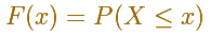
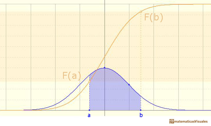
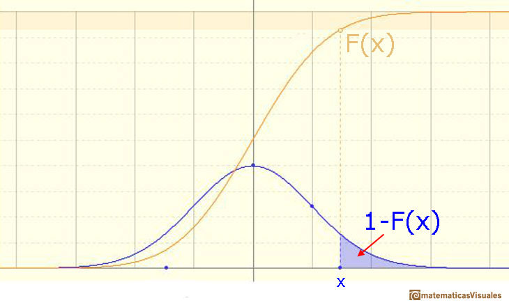
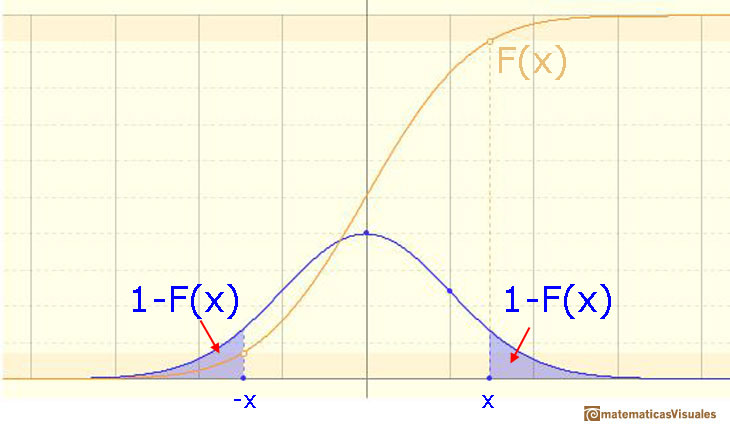
The (cumulative) distribution function of a random variable X, evaluated at x, is the probability that X will take a value less than or equal to x.

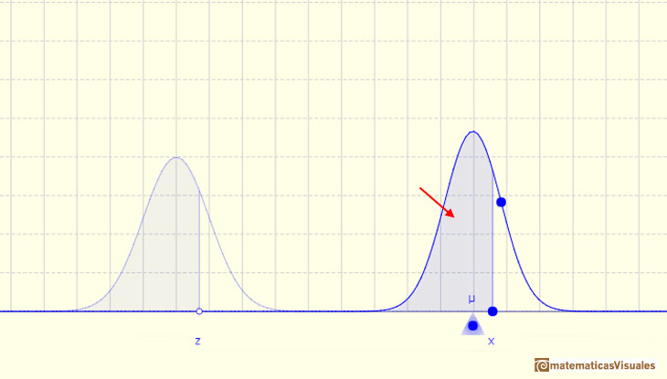
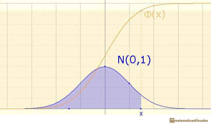
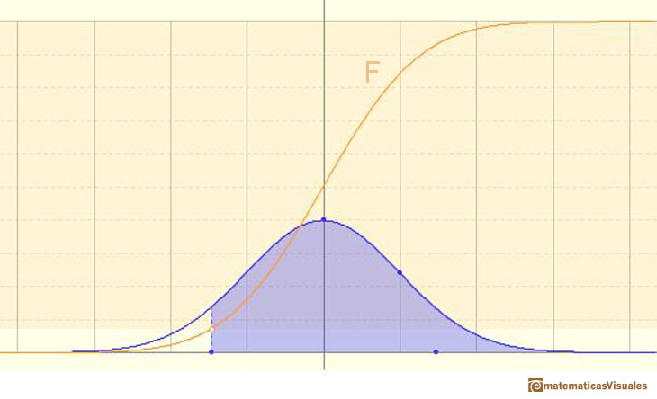
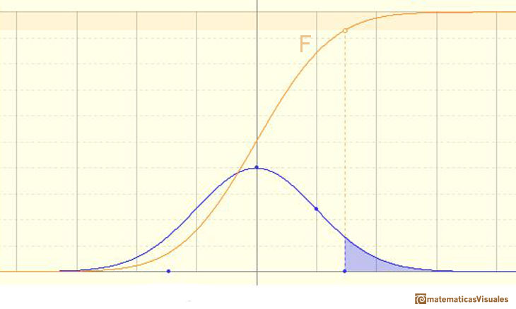
In the case of a continuous distribution (like the normal distribution) it is the area under the probability density function (the 'bell curve') from the negative left (minus infinity) to x. The shaded area of the curve represents the probability that X is less or equal than x.

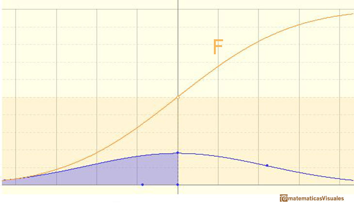
The (cumulative) ditribution function F is strictly increasing and continuous. It has an S-shape.

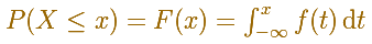
We can use the integral notation, then the (cumulative) distribution function can be written as an integral of its probability density function:

In the case of the normal distribution this integral does not exist in a simple closed formula. It is computed numerically.

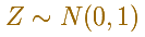
The Standard normal distribution plays an important role

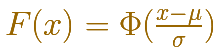
In some books they use a special notation for the (cumulative) distribution function in this special case of a standard normal distribution:

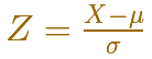
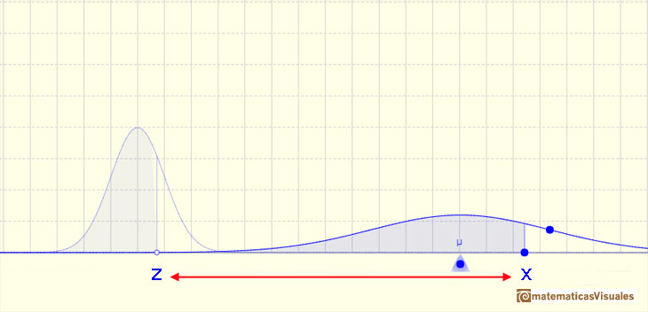
We already know that there is a relation between any normal distribution X and the standard normal distribution Z with mean 0 and standard deviation 1-

Normal Distributions: One, two and three standard deviations

One important property of normal distributions is that if we consider intervals centered on the mean and a certain extent proportional to the standard deviation, the probability of these intervals is constant regardless of the mean and standard deviation of the normal distribution considered.

This result is much more general: Any arbitrary normal distribution X can be converted to a standard normal distribution Z by changing variables to

You simply let the mean and variance of your random variable be 0 and 1, respectively.

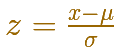
This is called standardizing the normal distribution. A value from any normal distribution can be transformed into its corresponding value on a standard normal distribution. You can standardize your value by subtracting the mean and dividing the result by the standard deviation (z-score).

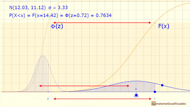
There is a practical consequence of that. We know that normal distributions are a family of infinite distributions and that to calculate probabilities we need to calculate integrals that we can do only numerically. But to do these calculations we only need one table of data or only one main function in any programing language (if we are using a computer). We need only to know the integral for the standard normal distribution.

We can calculate the probability of any interval:

The probability that the random variable falls within a given range is the area under the density function for that range. We use the (cumulative) probability function to do that.

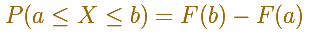
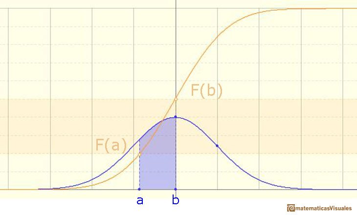
We can calculate more probabilities, for example:

An we can write:

MORE LINKS

Normal distributions

The Normal distribution was studied by Gauss. This is a continuous random variable (the variable can take any real value). The density function is shaped like a bell.

Poisson distribution

Poisson distribution is discrete (like the binomial) because the values that can take the random variable are natural numbers, although in the Poisson distribution all the possible cases are theoretically infinite.

Student's t-distributions

Student's t-distributions were studied by William Gosset(1876-1937) when working with small samples.

Calculating probabilities in t Student distributions (Spanish)

Binomial distribution

When modeling a situation where there are n independent trials with a constant probability p of success in each test we use a binomial distribution.

Normal approximation to Binomial distribution

In some cases, a Binomial distribution can be approximated by a Normal distribution with the same mean and variance.