
|
|

|

|


When modeling a situation where there are n independent trials with a constant probability p of "success" in each test we use a binomial distribution.
For example, if we toss n equal coins and we count heads as success, the probability of getting head can be any value between 0 and 1.
A binomial distribution is characterized by two parameters: n (a natural number) and p a number between 0 and 1.
If a random variable X follows the binomial distribution with parameters n and p, we write
The probability of getting exactly k successes in n trials is given by the probability mass function (or probability density function):
where
The later expression is known as the binomial coefficient, "n choose k", or the number of possible ways to choose k successes from n observations. The binomial coefficients form the rows of Pascal's triangle and can be calculated using factorials:
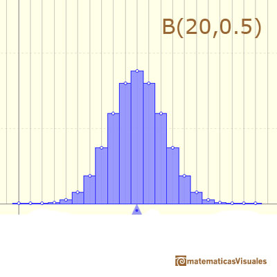
When p = 0.5 the probability mass function is symmetric:
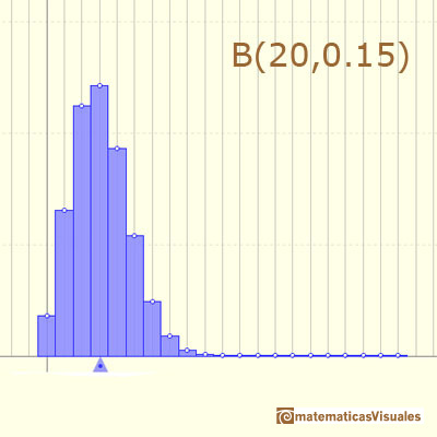
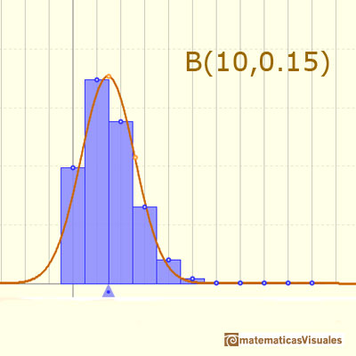
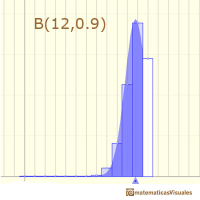
In other cases the function is asymmetric:
Mean and Variance of the Binomial Distribution are:
This applet is developed in HTML5 and can be managed using the mouse or the touchscreen of your tablet or mobile phone.
We can change the parameter n of the binomial distribution. The mean is represented by a triangle and it can be seen as a point of equilibrium. By dragging it we modify the mean and the parameter p.
Red points control vertical and horizontal scales.
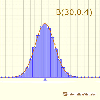
We can show a normal curve that has the same mean and variance as the binomial distribution.
In some cases, this normal curve is close to the binomial and can be used for calculations.
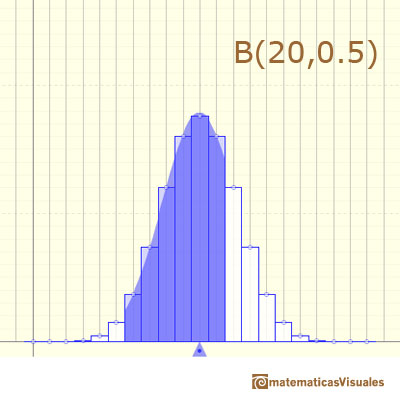
You can see why it is recommended to extend the interval for which you want to calculate the probability of the binomial in 0.5 above and below to use the normal distribution to approximate the probability (correction for continuity adjustement).
For example:

In other cases, this normal curve is not a good approximation to the binomial distribution:
Even with the correction for continuity adjustement the approximation is not accurate:
You can see more about the Normal approximation to the Binomial.
 NEXT
NEXT

MORE LINKS


